因子筛选:为什么样本内 1.95 的漂亮结果,样本外会归零 Factor screening: why an in-sample Sharpe of 1.95 can be worth zero
我把同一个「因子动物园」放进两档信噪比里跑了一遍:筛选的天花板由信噪比决定,不由方法决定。强信号下随便筛都对,弱信号下再多技巧也只是在噪声里挑噪声。 I ran the same factor zoo through two signal-to-noise regimes: the ceiling on screening is set by the signal, not by the technique.
TL;DR
- 弱信号下,"筛选"是幻觉。模拟中 400 个候选、8 个真因子(年化夏普 0.3)、15 年样本:按 t 值挑出的前 10 名,样本内夏普 1.95,样本外 0.03,命中率只有 30%。 With a weak signal, screening is an illusion: 400 candidates, 8 real (Sharpe 0.3), 15 years — the top-10 by t-statistic shows an in-sample Sharpe of 1.95 and 0.03 out of sample, with a 30% hit rate.
- 信号强的时候,方法差别不大。强信号档(300 个候选、12 个真、年化夏普 0.6)里,朴素筛选与更严格的流程结果几乎一样(样本外 1.63 vs 1.68)——所以不要用强信号的历史案例来证明你的流程好。 When the signal is strong, the method barely matters (out-of-sample 1.63 vs 1.68) — never use a strong-signal case to prove your process works.
- 多重检验的代价可以算出来。要证明一个年化夏普 0.3 的因子存在,在 400 次检验的阈值下需要约 164 年数据;即使只做一次检验也要约 43 年。(近似公式,见第三节) The cost of multiple testing is computable: proving a Sharpe-0.3 factor against 400 tests needs roughly 164 years of data; even a single test needs about 43.
- 真实世界的证据方向一致。文献给出的三件事:因子数量爆炸(Harvey–Liu–Zhu)、发表后收益衰减约一半(McLean–Pontiff)、大样本复制失败率很高(Hou–Xue–Zhang 等),而 2026 年的新论文把同样的问题带到了信用市场。 The literature points the same way: a factor explosion, roughly halved returns after publication, and high replication failure rates — extended to credit markets in 2026 work.
- 所以我不再"证明因子存在",而是回答"决策有多依赖它"。把单因子检验换成组合层边际贡献 + 收缩 + 敢说"这个我证不了"。 So the useful question is no longer "does this factor exist" but "how much does the decision depend on it".
本文实验是模拟:月度数据、alpha 恒定、噪声独立同分布,因此它只能说明"机制",不能代表真实市场的具体数字。事实性陈述(因子数量、发表后衰减、复制失败率)来自第四节列出的文献,链接均已核对可打开(核对日期 2026-09-25)。 The experiment is a simulation (monthly data, constant alpha, i.i.d. noise): it demonstrates a mechanism, not real-world magnitudes. Factual claims come from the sources in section 8, each link verified on 2026-09-25.
01为什么写这篇Why this note exists
做因子研究的人都会经历同一个瞬间:把 300 个候选因子丢进回测,按 t 值排序,取前 10 个,得到一个漂亮的夏普,然后拿它去讲一个故事。 Every factor researcher goes through the same moment: throw 300 candidates into a backtest, sort by t-statistic, keep the top ten, get a beautiful Sharpe, and tell a story about it.
问题在于:在同一份数据上挑选和评估,等于用同一张考卷出题又答题。挑选这一步本身就在消耗样本的信息量,而你最后看到的夏普里,混进了"挑"这个动作带来的运气。 The problem: selecting and evaluating on the same data is like writing and answering the same exam. The selection step consumes information from the sample, and the final Sharpe quietly includes the luck of having picked.
这篇想回答三个具体问题:弱的信号能被筛出来吗?强信号下筛选有没有价值?如果我必须给出一个数字,我该怎么算"我到底需要多少数据"? Three concrete questions: can a weak signal be screened out at all; is screening even valuable when the signal is strong; and if I had to give a number, how much data would I need?
文章的读法是这样的:第 2 节先把学术界的结论摆出来(谁测的、在什么口径下),第 3 节用两个模拟把机制演一遍,第 4 节把它变成一个可以手算的公式,最后三节是我实际怎么改流程、这套结论哪里不成立、以及我自己的判断。如果只读一节,读第 4 节——那一节的算术最容易被带进日常工作。 How to read it: section 2 gives the literature (who measured what, under which protocol), section 3 runs two simulations, section 4 turns it into arithmetic you can do by hand, and the last three sections cover process changes, limits and my own view.
02文献先把现实说清楚了What the literature already established
这不是我的新发现,学术界的结论比我狠得多。四组结果连起来是一条完整的证据链:[1][2][3][4][5] None of this is new: the academic results are harsher than my experiment. Four strands form one chain of evidence.[1][2][3][4][5]
| 结论Finding | 含义What it means | 来源Source |
|---|---|---|
| 因子数量爆炸,传统 t>2 门槛过低Factor proliferation; t>2 is too low | 候选越多,需要越高的显著性门槛;该文提出新的多重检验调整后门槛,量级明显高于 2More candidates require a higher bar; the paper proposes an adjusted threshold well above 2 | Harvey, Liu & Zhu[1] |
| 发表之后收益衰减Returns decay after publication | 样本外(发表后)收益平均约为样本内的一半,说明一部分"发现"来自数据挖掘而非真实定价错误Post-publication returns drop to roughly half of in-sample, evidence that part of the "discovery" was data mining | McLean & Pontiff[2] |
| 大规模复制的失败率很高Large-scale replication fails often | 在统一口径下重做大量异象,多数无法通过严格显著性检验;后续研究给出更乐观但同样苛刻的版本Re-running many anomalies under one protocol, most fail strict significance; later work is more constructive but equally demanding | Hou–Xue–Zhang;Jensen–Kelly–Pedersen[3][4] |
| 问题正在向其他资产蔓延The problem extends to other asset classes | 2026 年的新论文把"复制危机"搬到信用市场,并开始讨论因子之间共同定价的结构2026 papers move the replication question into credit markets and study co-pricing structure among factors | arXiv 2026[8][9] |
注:这些论文的结论不是"因子研究没用",而是"筛选标准必须与候选数量匹配"。 Note: the conclusion is not that factor research is pointless, but that the screening bar must match the number of candidates.
03我的实验:两档信噪比My experiment: two regimes
为了看清机制,我造了两个"因子动物园",每个因子都是月度收益序列,其中只有少数几个带真实的 alpha,其余全是噪声(带共同因子结构,所以因子之间有相关性簇)。样本内用来筛选,随后在未见过的样本外评估。[10] I built two simulated zoos of monthly factor series: a few carry genuine alpha, the rest are noise with a common-factor structure (so clusters exist). Selection happens in-sample; evaluation happens on unseen data.[10]
- 强信号档:300 个候选、12 个真、年化夏普 0.60、样本内 20 年Strong regime: 300 candidates, 12 real, annualised Sharpe 0.60, 20 years in-sample
- 弱信号档:400 个候选、8 个真、年化夏普 0.30、样本内 15 年(更接近真实的因子研究条件)Weak regime: 400 candidates, 8 real, annualised Sharpe 0.30, 15 years — closer to a real research setting
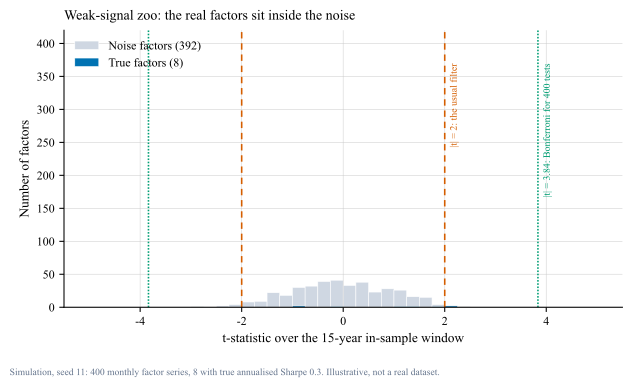
tools/make_figs_factor.py 可复现)。
真因子的 t 值区间是 0.23 ~ 2.20,而噪声因子的最大 |t| 达到 2.89——也就是说,没有任何一个真因子能达到"看起来显著"的位置,反而有噪声比真信号更显著。Bonferroni 门槛(400 次检验)是 |t| > 3.84,两边都过不了。
Real factors span t = 0.23–2.20, while the largest noise |t| reaches 2.89: no real factor looks significant, and some noise looks better than the truth. The Bonferroni bar for 400 tests is |t| > 3.84 — neither side clears it.接下来看四种做法在同一份模拟里的表现:全选、按 t 值取前 10(最常见的偷懒法)、五层过滤(下面第四节详述)、以及"上帝视角"(只用真因子,现实中不存在,作为上限参照)。 Four approaches, same simulated data: use everything, top-10 by t-statistic, a five-layer filter (section 4), and an oracle that keeps only the true factors as an upper bound.
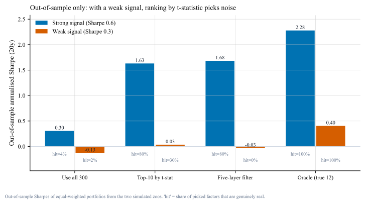
强信号档的对照很关键:300 个候选、12 个真、夏普 0.6 时,朴素筛选和五层过滤几乎一样(样本外 1.63 vs 1.68,命中率都是 80%)。结论:方法的价值只在弱信号区显现,而真实世界恰恰是弱信号区。如果你只能用强信号的历史案例来证明流程有效,那你其实什么都没证明。 In the strong regime the naive and layered rules are indistinguishable (1.63 vs 1.68, both 80% hit). The method only matters in the weak regime — which is where real research lives. A process demonstrated only on strong-signal history demonstrates nothing.
把两张图放到一起看
图 1 说的是"信号在哪里":真因子和噪声完全混在一起,你无法只靠眼睛把它们分开。图 2 说的是"结果会怎样":在弱信号档里,按 t 值取前 10 得到的样本外夏普只有 0.03,而"上帝视角"(只用真因子)也只有 0.40。两句合起来是一个让人不太舒服的结论——不是你的筛子差,而是这片地质本来就没有多少金子,所以"筛出 0 个"有时就是正确答案。 Figure 1 shows where the signal sits (mixed into the noise); figure 2 shows what follows (an out-of-sample Sharpe of 0.03 for the naive pick, and only 0.40 for the oracle). Together they say the problem is not a weak sieve but thin ore — and "picking nothing" is sometimes the correct answer.
04证明一个因子存在,需要多少年数据How much data does proof need
多重检验的代价可以算出来。用 t 统计量与年化夏普之间的近似关系 t ≈ SR × √年数,反解就得到"达到显著所需要的年数" = (t 门槛 / SR)²。 The cost is computable. Using the approximation t ≈ SR × √years, the data needed is (threshold / SR)².
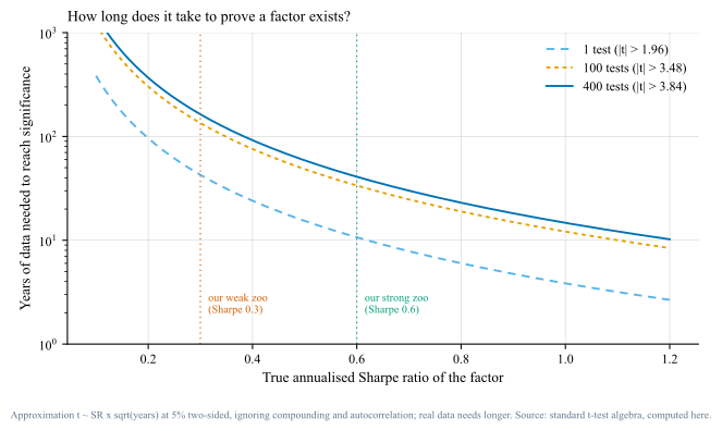
手算一遍:164 年是怎么来的
这一步值得自己推一遍,因为它只用到中学统计。年化夏普为 SR 的策略,在 T 年样本上的 t 统计量约等于 t ≈ SR × √T。要对抗 n 次检验,5% 双尾的 Bonferroni 门槛是 t* = Φ⁻¹(1 − 0.05/(2n))。把 400 次检验代进去得到 t* ≈ 3.84;再令 SR × √T ≥ 3.84,解出 T ≥ (3.84 / 0.3)² ≈ 164 年。如果这个因子其实是 0.6 的夏普,同一门槛只需要 41 年;如果连多重检验都不做(n = 1,t* ≈ 1.96),0.3 的夏普也要 43 年。这三个数字连起来说明:长度不足时,"没通过检验"和"不存在"是两件事。
Worth doing by hand: for annualised Sharpe SR over T years, t ≈ SR × √T. Against n tests the Bonferroni bar is t* = Φ⁻¹(1 − 0.05/2n), which is about 3.84 for 400 tests. Solving gives T ≈ (3.84/0.3)² ≈ 164 years; with Sharpe 0.6 it drops to 41 years, and with no multiple-testing correction (n = 1, t* ≈ 1.96) a Sharpe-0.3 factor still needs 43 years. Failing a test and not existing are different things.
05那我实际怎么做What I actually do about it
实验跑完,我把自己的流程改成下面五条。它不是"更好的筛子",而是承认单因子检验的能力上限之后的替代做法。 Five changes to my own workflow. Not a better sieve — a response to the limits of single-factor testing.
- 先写经济故事,再看数据。候选因子的来源先要有机制解释(风险补偿、行为偏差、制度约束);没有故事的因子即使 t 值高也进不了池子——这是最低成本的事前筛选。 Economic story first. A candidate needs a mechanism (risk premia, behaviour, constraints) before any data. No story, no entry — the cheapest filter available.
- 把"筛选"换成"组合层边际贡献"。不看单因子的 t 值排名,而是问:把它加进现有组合,夏普/回撤/换手各变化多少?这直接对应决策,而不是对应统计显著性。[5] Replace screening with portfolio marginal contribution. Ask what changes in Sharpe, drawdown and turnover when the factor joins the book — a decision question rather than a significance question.[5]
- 用收缩,而不是硬选。与其在"留下/丢弃"之间二选一,不如给所有候选一个按证据强度缩减的权重(贝叶斯收缩 / 岭回归),让弱证据自带惩罚。 Shrink instead of selecting. Rather than keep-or-drop, weight every candidate by the strength of its evidence (Bayesian shrinkage, ridge), so weak evidence penalises itself.
- 对多重检验诚实定价。报告筛选过程本身:试了多少个变体、用什么门槛、如果按 Bonferroni 或 Deflated Sharpe Ratio 折算,结论还剩多少。[7] Price the multiple testing honestly. Disclose the search: how many variants, which bar, and what survives after a Bonferroni or Deflated-Sharpe adjustment.[7]
- 敢说"这个我证不了"。当样本量根本不足(如图 3 的 164 年),正确回答不是编一个理由,而是承认不确定性,并改用对结论影响更小的决策——例如降低仓位而不是全押。 Say "I cannot prove this". When the data is simply insufficient (see the 164 years), the honest answer is to admit it and make a decision that depends less on the claim — smaller size instead of full conviction.
06局限与反方观点Limits and the other side
- 我的实验是模拟,不是市场。alpha 恒定、噪声独立、没有制度变迁与拥挤度变化。现实中真因子的 alpha 会衰减,所以弱信号档的"五层过滤全军覆没"在真实世界里可能更糟,也可能因为经济机制的存在而更好——模拟给不出答案。 The experiment is a simulation. Constant alpha, i.i.d. noise, no regime change or crowding. Real alphas decay; the real-world outcome could be worse — or better, if genuine mechanisms exist.
- 文献本身有分歧。以复制失败率为例,Hou–Xue–Zhang 的口径偏严格(微观市值、等权),Jensen–Kelly–Pedersen 用不同的检验框架得到的可复制比例明显更高。引用单一结论是危险的。[3][4] The literature disagrees. Replication failure rates depend on protocol (microcaps, equal weighting) versus a different testing framework that finds much higher replicability. Quoting one side is dangerous.[3][4]
- 图 3 是近似。t ≈ SR√年数 忽略了复利、自相关与偏度;若收益有自相关,实际所需样本更长。它的用途是给出量级感,不是精确答案。 Figure 3 is an approximation. It ignores compounding, autocorrelation and skew; autocorrelated returns need longer. Use it for orders of magnitude, not precision.
- 反方观点:不筛选更危险。如果因为"筛不出来"就什么都不做,组合会被噪声稀释——实验里"全选"的样本外夏普在弱信号档是 −0.13。正确姿态是收缩与分散,而不是放弃。 The other side: not screening is worse. Using everything gave −0.13 out of sample in the weak regime. The answer is shrinkage and diversification, not surrender.
三个常见误解
- "提高门槛就能解决。"门槛只能减少误选,不能创造信息。当真因子的 t 值(0.23–2.20)低于噪声的最大值(2.89)时,再高的门槛也只会把所有东西一起筛掉——这就是弱信号档里五层过滤命中 0 个的原因。 "A higher bar fixes it." A bar reduces false picks; it does not create information. When true factors sit below the noisiest noise, raising the bar removes everything at once.
- "换了机器学习就不一样。"机器学习改变的是"如何组合信息",不改变"信息有多少"。因子动物园的问题本质是样本量与候选数之比,换模型不改变这个比值。 "Machine learning changes the picture." ML changes how information is combined, not how much exists; the ratio of sample size to candidate count is unchanged.
- "样本外归零说明信号是假的。"不一定。可能是信号真实但被成本、容量或拥挤度吃掉了;也可能是样本外恰好处在不利制度。正确的表述是"现有证据不足以支持这个仓位",而不是"这个规律不存在"。 "Zero out of sample means the signal is fake." Not necessarily: it may be real but eaten by costs, capacity or crowding — or simply out of regime. Say "the evidence does not yet support the position", not "the pattern does not exist".
07我的判断My take
我认为"因子筛选"这个词误导了很多人:它听起来像是从沙子里挑金子,但大多数时候我们面对的是一堆看起来都像金子的沙子。实验里弱信号档的五层过滤选出 4 个因子、命中 0 个——这不是因为流程写得差,而是因为在那个信噪比下,任何流程都做不到。 "Factor screening" misleads: it sounds like picking gold from sand, when usually the sand all glitters. In the weak regime the layered filter picked four factors and none were real — not because the process was sloppy, but because at that signal-to-noise nothing would work.
所以我把研究目标从"证明某个因子存在"改成"我的决策有多依赖这个结论"。后者可以回答,前者往往不能。面试里我更愿意说:这个信号我测过,样本量对应到图 3 大约是 40 年,我手上只有 15 年,所以我只给它小仓位——而不是说它夏普 1.95。 So my research question changed from "does this factor exist" to "how much does my decision depend on it". The first is usually unanswerable; the second is answerable — and is what I would say in an interview, rather than quoting a Sharpe of 1.95.
08来源(链接均于 2026-09-25 核查)Sources (links verified 2026-09-25)
- Harvey, C. R., Liu, Y., & Zhu, H. (2016). … and the Cross-Section of Expected Returns. Review of Financial Studies. doi.org/10.1093/rfs/hhv059 (DOI 已用 Crossref 核对;出版社页面会拦截自动访问,浏览器可正常打开)
- McLean, R. D., & Pontiff, J. (2016). Does Academic Research Destroy Stock Return Predictability? Journal of Finance. doi.org/10.1111/jofi.12365
- Hou, K., Xue, C., & Zhang, L. (2020). Replicating Anomalies. Review of Financial Studies. doi.org/10.1093/rfs/hhy131 · 公开复制数据:public replication data: global-q.org/factors.html
- Jensen, T. I., Kelly, B., & Pedersen, L. H. (2023). Is There a Replication Crisis in Finance? Journal of Finance. doi.org/10.1111/jofi.13249
- Feng, G., Giglio, S., & Xiu, D. (2020). Taming the Factor Zoo: A Test of New Factors. Journal of Finance. doi.org/10.1111/jofi.12883
- Gu, S., Kelly, B., & Xiu, D. (2020). Empirical Asset Pricing via Machine Learning. Review of Financial Studies. doi.org/10.1093/rfs/hhaa009
- Bailey, D. H., & López de Prado, M. (2014). The Deflated Sharpe Ratio: Correcting for Selection Bias, Backtest Overfitting and Non-Normality. Journal of Portfolio Management. doi.org/10.3905/jpm.2014.40.5.094 (该 DOI 经 Crossref 核对存在)
- arXiv (2026-04). The Corporate Bond Factor Replication Crisis. arxiv.org/abs/2604.07880
- arXiv (2026-04). The Co-Pricing Factor Zoo. arxiv.org/abs/2604.04430
- arXiv (2023-11). Forking Paths in Financial Economics(研究自由度与多重检验). arxiv.org/abs/2401.08606
- 本文实验代码:
tools/make_figs_factor.py(固定随机种子,可完全复现;模拟设定见第三节)。
09分享版摘要Shareable summary
10引用本文Cite this note
Aylon (2026). 因子筛选:为什么样本内 1.95 的漂亮结果,样本外会归零. Notes, v1.0. https://aayloo.github.io/notes/factor-screening/
11更新日志Changelog
| 版本Version | 日期Date | 改动Change |
|---|---|---|
| v1.0 | 2026-09-25 | 初版。两档信噪比模拟 + 11 条来源(链接已核查)。 First version: two-regime simulation and eleven verified sources. |