约束的代价:多资产组合里,每个"不许超"都在收费 Every constraint has a price
在同样的 8% 波动预算下,四条典型机构约束一共拿走 46.8 bps 的预期收益/年。但故事的另一半是:当你手上的样本很短时,同样的约束不是成本,而是保险——它挡住的是估计误差,不是市场。 At an identical 8% volatility budget, four ordinary institutional constraints cost 46.8 bps a year of expected return. The other half of the story: when your sample is short, the same constraints act as insurance against estimation error.
TL;DR
- 无约束的"最优"很吓人。同样 8% 波动预算下,模型把 63.8% 押在信用债、18% 在 REITs、13.9% 在新兴市场股票——这不是洞察,这是误差放大器。 The unconstrained optimum puts 63.8% in credit at an 8% volatility budget — an error amplifier, not an insight.
- 四条约束合计 46.8 bps/年:单资产上限 20%(27.9)、久期上限 2 年(7.0)、月度换手上限 25%(13.5)、禁投清单(10.1)。但不是简单相加——四条单价算术和是 58.5,合起来只有 46.8,因为约束之间会互相遮蔽。 The four constraints cost 46.8 bps in total, against 58.5 bps if added up naively — constraints mask each other.
- 每条约束的价格取决于它"最后"值多少钱。从全约束组合里单独拿掉换手上限,收益一分钱都不多(+0.0 bps)——它在其他三条存在时已经不起作用了。 A constraint is worth what it costs last: removing the turnover cap from the fully constrained portfolio adds nothing.
- 收紧上限是非线性的。从 60% 收到 40% 只要 8.7 bps,从 20% 再收到 16% 要 39.4 bps。而且 16% 已接近可行下限(7 个资产时低于 1/7 ≈ 14.3% 在数学上就无解)。 Tightening is non-linear, and with seven assets a cap below 1/7 is simply infeasible.
- 样本越短,约束越是保险。30 条随机路径:估计窗口只有 24 个月时,无约束组合的样本外超额夏普 10 分位是 −0.02,全约束组合是 +0.18;样本拉长到 240 个月,两者收敛(0.41 vs 0.42)。 With a 24-month estimation window the 10th-percentile out-of-sample Sharpe is −0.02 unconstrained versus +0.18 constrained; at 240 months they converge.
本文用7 个资产、年化参数设定的模拟(股票 7%/16%、国债 3.5%/5%、信用债 5%/7%、黄金 4%/14%、REITs 7.5%/18%、新兴市场 8%/20%、现金 2%),基准组合是满足全部约束的政策组合。数字来自模拟,不是任何真实组合的历史业绩;它说明的是机制与量级,不是市场的具体答案。代码:tools/make_figs_constraints.py(固定种子)。
A simulated seven-asset universe with stated annual parameters; the benchmark policy portfolio is compliant with every constraint. Numbers illustrate a mechanism and its scale, not real portfolio history. Code included, fixed seed.
01会议上的那句话The sentence in the meeting
"单资产不超过 20%,久期不超过 2 年,月度换手控制在 25% 以内,新兴市场先别碰。" "No single asset above 20%, duration under two years, monthly turnover below 25%, and stay out of emerging markets."
这几句话在投委会里从不引起争论,因为每一条听起来都合理,都是风控语言。但没人说出它们的价格。结果通常是:模型给出的权重被手工"修一修",一年后跟基准比,说不清是判断对了还是被约束磨平了。 Nobody argues with these sentences — each sounds prudent. But nobody says what they cost. The weights get hand-adjusted, and a year later nobody can tell whether the view paid off or the constraint sanded it away.
这篇想做的就是把价格算出来:在同样的风险预算下,每条约束、以及它们合在一起,究竟拿走多少预期收益。 This note prices them: at a fixed risk budget, how much expected return does each constraint — and all of them together — actually take?
读的时候只需要抓住一件事:本文所有的"代价"都是相对量——相对于 8% 的波动预算、相对于一个已经合规的基准组合、相对于当下的约束清单。换一组前提,数字会完全不一样,但比较的方法是一样的,这也是我最希望读者带走的部分。下面每一节都先给结论,再讲为什么。 One thing to hold on to: every cost here is relative — to an 8% volatility budget, to a compliant benchmark, and to the current list of constraints. Change the premises and the numbers change; the way of comparing them does not.
02先把"无约束最优"亮出来Look at the unconstrained optimum first
实验的统一口径是:波动不超过 8%,在此前提下最大化预期收益。这个口径比"最大化夏普"更接近机构实务(风险预算先定,收益尽量争取),也避免了"全押现金"这类退化解。 The common yardstick: maximise expected return subject to volatility ≤ 8%. This mirrors institutional practice — the risk budget comes first — and avoids degenerate solutions.
| 资产Asset | 无约束最优Unconstrained | 全约束Constrained |
|---|---|---|
| 股票Equities | 0.0% | 20.0% |
| 国债Govt bonds | 0.0% | 17.1% |
| 信用债Credit | 63.8% | 20.0% |
| 黄金Gold | 4.2% | 20.0% |
| REITsREITs | 18.0% | 20.0% |
| 新兴市场EM equities | 13.9% | 0.0% |
| 现金Cash | 0.0% | 2.9% |
| 预期收益Expected return | 5.83% | 5.36% |
| 组合久期Portfolio duration | 2.55 年 | 1.83 年 |
先看左边这列:模型把六成资金压在一个资产上。这不是因为它更了解信用债,而是因为它对预期收益的估计太自信——这正是 Michaud 1989 说的"优化器是误差放大器"。[1] The left column is the point: 64% in one asset, not because the model knows credit better, but because it trusts its own point estimates.[1]
怎么读表 1
看两列之间的差别,比看两列的绝对值更有信息量。第一,信用债从 63.8% 被压到 20%——那条上限切断的正是模型最爱下注的地方。第二,股票从 0% 被动升到 20%:模型原本根本不想要股票,是上限把资金"挤"过去的,这属于约束的副作用,不是模型的观点。第三,久期从 2.55 年降到 1.83 年,下降的部分来自久期上限,而不是优化器主动选择更短的久期。这三处变化合起来,才是"46.8 bps"的来历。 Read the difference between the columns, not the levels. Credit is capped from 63.8% to 20% — the cap cuts exactly where the optimiser wanted to bet. Equities rise from 0% to 20% because the cap pushes money there: a side effect, not a view. Duration falls from 2.55 to 1.83 years because of the duration cap, not because the optimiser prefers it.
03每条约束的价格The price of each constraint
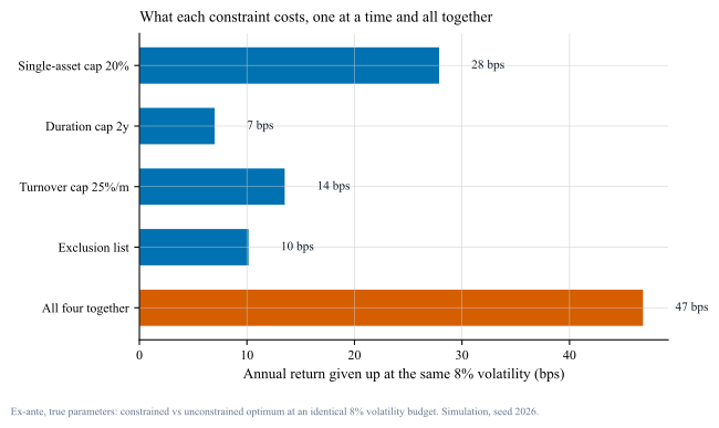
tools/make_figs_constraints.py)。
蓝色是单条约束单独施加,红色是四条一起。注意最后那根柱子:四条一起拿走 46.8 bps,小于四条单价的算术和 58.5 bps——约束彼此会遮蔽。
Blue: each constraint alone. Red: all four. The total, 46.8 bps, is below the arithmetic sum of 58.5 — the constraints overlap.- 单资产上限 20%:27.9 bps——四项里最贵的一组,因为它直接切断"集中押注"的能力。 Single-asset cap 20%: 27.9 bps — the most expensive, because it removes concentration precisely where the optimiser wants it.
- 月度换手上限 25%:13.5 bps——它的价格取决于你从哪里出发。基准组合与最优解差得越远,这条约束越贵。 Turnover cap 25%: 13.5 bps — priced relative to the starting portfolio; the further the optimum, the costlier the cap.
- 禁投清单(去掉新兴市场):10.1 bps——删掉一个资产等于删掉一维自由度,价格不高但不可逆。 Exclusion list: 10.1 bps — deleting an asset removes a degree of freedom: cheap here, but irreversible.
- 久期上限 2 年:7.0 bps——最便宜的一条,因为它只在优化器想把久期拉长时才咬人。 Duration cap 2y: 7.0 bps — the cheapest, because it only bites when the optimiser wants duration.
把 27.9 bps 翻译成钱
bps 这个词容易让人麻木,换成钱会清楚很多:对一个 10 亿港元的组合,27.9 bps ≈ 每年 279 万港元的预期收益;四条约束加总 46.8 bps ≈ 468 万港元。要提醒两点:这是预期收益的差,不是每年必然发生的损失,某些年份完全可能因为约束而少亏;而且它衡量的是"理论代价",在样本很短、参数不可信的场景里,同一组约束的净效果可能是正的(见第 6 节)。 bps numbs the senses; money does not. On a HKD 1bn book, 27.9 bps is about HKD 2.79m of expected return a year, and all four constraints together about HKD 4.68m. Two caveats: this is a difference in expected return, not a guaranteed annual loss, and in short-sample settings the same constraints can be worth more than they cost (section 6).
04约束之间会互相遮蔽Constraints mask each other
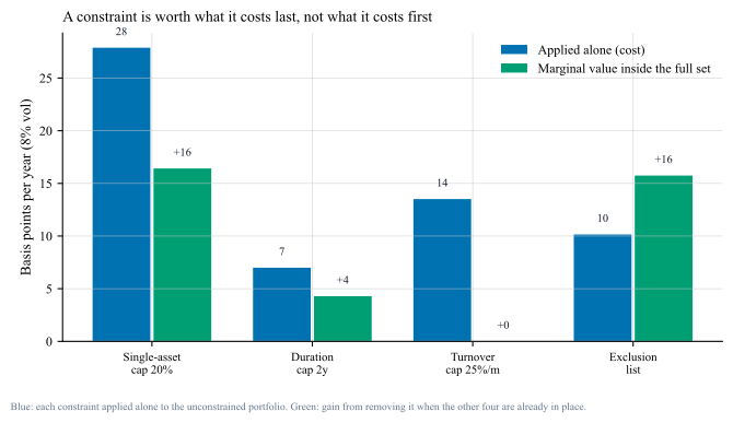
这意味着"逐条评估约束"是错的方法。正确的问法是组合层面的边际:把候选约束集当成一个包裹,用"逐条加入"和"逐条移除"两个方向各跑一遍,看价格在哪个方向出现。如果两条约束指向同一个方向(比如上限与换手),第二条几乎必然便宜——但这不代表它没用,在极端行情里它可能是唯一有效的那条。 Evaluating constraints one by one is the wrong method. Ask the portfolio-level marginal: add each constraint, then remove each from the full set. Two constraints pulling the same way guarantee a cheap second addition — which does not make it useless under stress.
05收紧上限是非线性的Tightening is not linear
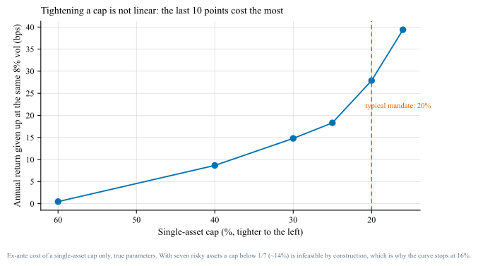
06但样本短的时候,约束是保险With short samples, constraints are insurance
上面全是"用真实参数算出来的代价"。现实中你并不知道真实参数,只能从历史里估。这时结论会翻转一部分——这就是 Michaud 与 Jagannathan & Ma 之间的张力:一位说约束有害,另一位说"错误的约束反而有用"。[1][2] Everything above is priced with true parameters. In practice you estimate them from history — where a different result appears: Michaud says constraints hurt, Jagannathan & Ma show wrong constraints often help.[1][2]
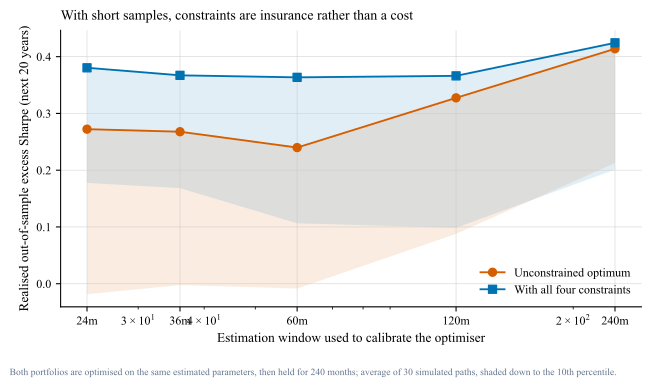
这解释了一个常见困惑:为什么"回测里约束拖累业绩",而"实盘里加了约束反而更稳"。两个说法都对——只是在用不同的样本长度说话。 This resolves a common paradox: constraints look like a drag in backtests and like ballast in live portfolios. Both are right — they are just measured on different sample lengths.
07所以我在实际工作里怎么做What I actually do
- 先报价格,再谈约束。任何约束提案都附一句"在我们 8% 风险预算下约值 X bps"——这句话让讨论从偏好变成取舍。 Price it before you debate it. Every constraint proposal carries a line: about X bps at our risk budget.
- 用包裹定价,不用逐条定价。报告"逐条加入"和"逐条移除"两个方向——只报一个方向会系统性高估约束的代价。 Price the package, not the items. Report both add-one and remove-one margins; a single direction overstates the cost.
- 约束要按"它挡住什么"来设计,而不是按习惯。挡集中度用上限,挡误差放大用收缩与上限,挡流动性用换手,每家机构的约束清单应该长短不一。 Design constraints by what they block. Caps block concentration, shrinkage and caps block error amplification, turnover limits block liquidity risk.
- 先查可行性再上会。1/n 这道小学算术能挡掉一部分提案(n 是可选资产数)。 Check feasibility first. The arithmetic of 1/n, with n the number of eligible assets, kills some proposals before the meeting.
- 样本短时,把约束当成不确定性预算来管:与其纠结"要不要加 20% 上限",不如问"我凭什么相信 64% 这个数字"。[3] With short samples, treat constraints as an uncertainty budget. The real question is not the cap; it is why anyone believes 64%.[3]
08局限与反方观点Limits and the other side
- 参数是我设的。预期收益、波动与相关矩阵都是假设,换一组数字,bps 会变。这篇文章的价值在方法(怎么定价、怎么读边际),不在具体数值。 The parameters are mine. Change them and the bps change. The contribution is the method, not the numbers.
- 没有交易成本与税。换手上限的真实价值部分来自成本节省,本文的换手代价只算收益维度,因此低估了换手上限的合理性。 No costs or taxes. Part of the value of a turnover limit is the cost it saves, which is outside this measurement.
- 约束的价值有很大一部分是"防人"而不是"防模型"。禁投清单、单资产上限常来自合规与委托要求,这时候谈 bps 只是让代价可见,不是否定约束。 Much of a constraint's value is governance, not modelling. Pricing them makes the cost visible without arguing them away.
- 反方:为什么不干脆别用优化器?1/N 在文献里常常打赢样本内最优的均值方差组合,而且不需要估计参数。这确实是本文结论的自然延伸——如果你的参数估计不够好,约束或等权是同一件事的两种说法。[4] The other side: why use an optimiser at all? 1/N often beats in-sample mean-variance with no parameter estimation.[4]
三个常见误解
- "约束越少越好。"不对。本文第 6 节显示,估计窗口越短,约束带来的样本外保护越明显(10 分位从 −0.02 提到 +0.18)。约束多不等于差,约束与你的参数质量不匹配才差。 "Fewer constraints is better." No: with short estimation windows, constraints improved the 10th-percentile outcome from −0.02 to +0.18. What hurts is a constraint set that does not match the quality of your estimates.
- "代价不大就无所谓。"46.8 bps 听起来很小,但它对抗的是夏普 0.5–0.6 这个量级的策略——它相当于吃掉约 8%–9% 的预期超额收益。在长期复利里,这类"看起来很小"的数字才是最终决定成败的那一批。 "The cost is too small to care about." 46.8 bps against a Sharpe of 0.5–0.6 is roughly 8–9% of expected excess return — the kind of small number that compounds into the final answer.
- "算这个是为了删掉约束。"不是。合规、委托与治理类约束不该被 bps 论证掉;把它们定价的目的是让取舍变得可见——知道价格之后,会议讨论的就不再是"我觉得",而是"我们愿意为这条约束付多少"。 "Pricing constraints is an argument for removing them." No. Mandate and governance constraints should not be argued away by bps; pricing them makes the trade-off visible so the discussion becomes "how much are we willing to pay for this rule".
09我的判断My take
我认为"约束的代价"这个说法本身就容易误导:约束不是免费的,但它也不是纯粹的损耗——它买到的是对你自己估计误差的保险。样本越长、对参数越有信心,这份保险越贵;样本越短、模型越自信,这份保险越值。 "The cost of constraints" is itself misleading: a constraint is not a pure loss — it buys insurance against your own estimation error. The longer your sample, the dearer the insurance; the shorter it is, the more it is worth.
所以我在会上只会说一句:"这条约束值 28 bps,它挡住的是我们把 64% 押在一个资产上的风险——如果你们认为那个 64% 靠得住,我们就该删掉它;如果不确定,那就留着。"把偏好问题翻译成价格问题,是我从这套实验里学到的最有用的东西。 So the sentence I would use: this constraint costs 28 bps and it blocks a 64% bet; if you believe the 64%, remove it; if not, keep it. Turning a preference into a price is the practical lesson.
10来源(链接均于 2026-09-29 核查)Sources (links verified 2026-09-29)
- Michaud, R. O. (1989). The Markowitz Optimization Enigma: Is 'Optimized' Optimal? Financial Analysts Journal. doi.org/10.2469/faj.v45.n1.31
- Jagannathan, R., & Ma, T. (2003). Risk Reduction in Large Portfolios: Why Imposing the Wrong Constraints Helps. Journal of Finance. doi.org/10.1111/1540-6261.00580 · 免费工作论文版:free working paper: NBER w8922
- Black, F., & Litterman, R. (1992). Global Portfolio Optimization. Financial Analysts Journal. doi.org/10.2469/faj.v48.n5.28
- DeMiguel, V., Garlappi, L., & Uppal, R. (2009). Optimal Versus Naive Diversification. Review of Financial Studies. doi.org/10.1093/rfs/hhm075
- Clarke, R., de Silva, H., & Thorley, S. (2011). Minimum-Variance Portfolio Composition. Journal of Portfolio Management. doi.org/10.3905/jpm.2010.2010.1.009
- arXiv (2026-07). Fragility of Minimum-Variance Portfolios. arxiv.org/abs/2607.18624
- arXiv (2026-09). Decision-Focused Learning for Mean-Variance Portfolio Optimization via KKT-Based Reformulation. arxiv.org/abs/2609.21427
- 本文实验代码:
tools/make_figs_constraints.py(固定种子;模拟设定见开头「口径」)。
11分享版摘要Shareable summary
12引用本文Cite this note
Aylon (2026). 约束的代价:多资产组合里,每个"不许超"都在收费. Notes, v1.0. https://aayloo.github.io/notes/cost-of-constraints/
13更新日志Changelog
| 版本Version | 日期Date | 改动Change |
|---|---|---|
| v1.0 | 2026-09-29 | 初版:7 资产模拟、四张图、8 条来源(链接已核查)。 First version: seven-asset simulation, four figures, eight verified sources. |